DEq - The Math#
DEq models the marginal win rate attributable to drafting a card versus replacing it with a basic land. Under simplified assumptions, detailed below, the base formula for DEq can be explicitly derived and looks like this:
To better model expected selection biases and movements in the metagame, I add two adjustment terms, which are both relatively minor in comparison with the base formula above. DEq Base is perfectly suitable on its own as a card quality metric. Before moving on, let me collect the free parameters of the DEq formula here along with their current values, for reference.
ATA 1.0 pick equity \(r_1 = 3.0\%\)
Cards per pack \(K = 14\)
Bias adjustment coefficient \(\beta = 1.0\)
Daily metagame mean-regression rate \(\lambda = 0.95\)
Daily games played decay rate \(\gamma = 0.95\)
Card DEq impact of metagame decay \(L = 0.6\)
All-player game sample weight \(M = 1000\)
Pick Equity#
Let
be the theoretical mean game win rate for a given player cohort (e.g. me, you, or 17Lands “Top” players) for a metagame (e.g. a particular set on a particular day for a particular rank), and let
be the probability of winning conditioned on a “null pick” \(N_k\), meaning, picking a card straight into the trash, or replacing it with a basic land, for one \(k\)-th pick in one pack (i.e. averaged over the three packs). Then let
be the “pick equity” of a \(k\)-th pick, that is, the marginal win rate attributable to making that pick, on average. When you choose a card with a \(k\)-th pick, on average, you are giving up \(r_k\) of winrate in exchange for adding that particular card to your pool.
A proper estimate of \(r_k\) is a piece of analysis that I intend to do thoroughly down the road, but for now I am relying on estimates based on previous analysis and a bit of eye test on the final results. I’ve found that a quadratic fit with P1 being worth 3% gives good results. Note that DEq is most useful in pack one, where your early picks are generally more valuable.
import matplotlib.pyplot as plt
import matplotlib.ticker as mtick
import numpy as np

_, ax = plt.subplots()
x = np.arange(1, 15)
y = 0.03 * (1 - (x - 1) / 14) ** 2
ax.yaxis.set_major_formatter(mtick.PercentFormatter(1.0, decimals=1))
ax.plot(x, y)
ax.set_title("Model Pick Equity by Pick Num")
ax.set_ylabel("Pick Equity")
ax.set_xlabel("Pick Num")
ax.set_xticks(x)
plt.show()
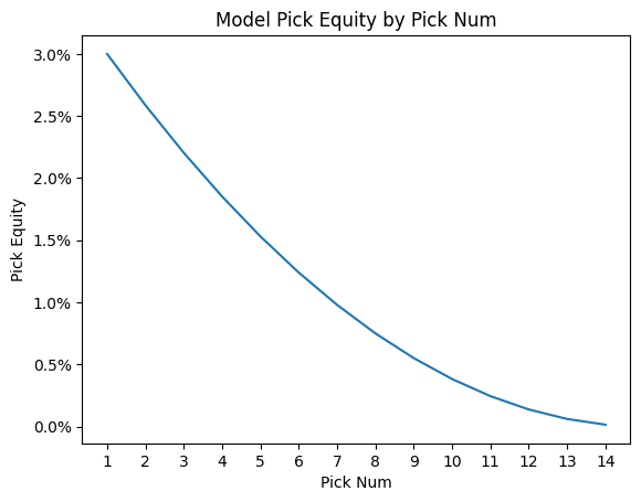
In practice, we apply this model to the observed ATA (average taken at), since that is the number we have available. While there is a bit of convexity, this shouldn’t trouble us too much. For a given card, in a given metagame, we identify the pick equity of the card as \(\text{PEq}(c) = r_{\text{ATA}(c)}.\)
DEq Base#
We’re going to get technical because it will allow us to specify exactly the assumptions that create bias in the final model. The notation is a bit complicated, and could be improved, but sometimes that’s just the way it is. The final formula is relatively intuitive so you can skip to that. The essence of the below is that DEq is GP WR plus Pick Equity modified by GP %. We will have to define a bunch of events and rearrange some conditional probabilities to get there.
Recall that \(P\) represents a particular player/metagame probability model, and a conditional like \(P[X| A]\) effectively takes a weighted average of \(X\) restricted to the (theoretical) observations of \(A\) within that same model. \(P\) is “omniscient” in that it gives the true rate of outcomes all possible events. Finally, \(P\) is a measure on “pick events”, that is, observations of individual draft picks coupled with the resulting outcome.
Given a card \(c\), let \(C\) be the set of draft pick events \(\omega\) where \(c\) was selected.
Now when we define our own probability space, we can make the event space as detailed as we like, so we couple the elements \(\omega\) with all the information needed to construct counterfactual scenarios, and we will rely on \(P\) to average them correctly. So let \(\tilde{W}\) represent the counterfactual outcome under the null pick, and let
This is the formal expression of our idea about marginal win rate. We properly ask, at the operative moment, “What happens if we don’t take the card instead?” So \(q(c)\) is what I call the “draft equity” of \(c\), and \(DEq\) will be the metric estimating \(q\).
It will be more convenient to express this using the null pick notation above, so we “split out” the counterfactual outcomes to new elements \(\omega\) to create events \(N_C\) representing the same scenario up to the pick event, which is then replaced with the null pick and followed to the counterfactual outcome. Then
\(N_C\) may have zero measure under \(P\), but we can just stipulate that events are weighted according to \(C\) in the conditional measure and that should handle it.
Now the available metric that most nearly estimates \(P[W | C]\) is GP WR, “games-played win rate”, under the further condition that \(c\) is played in our deck. Let \(D = D(\omega)\) be the event that the card resulting from the specific pick event \(\omega\) is played in the deck, and write
Now
To break this down we need some assumptions, which we will write down.
Assumption 1: The quality (winrate) of \(\omega \in N_C\) is independent of the card \(c\), and only depends on the pick equity lost to the null pick. We should have good reason to believe this is not the case. We will look at a first attempt to adjust for the bias caused by this assumption in the next section.
Assumption 2: The quality of \(\omega \in C \cap D^c\) is independent of \(c\), and depends on the pick equity given up by not playing \(c\). Again, this shouldn’t be strictly true. We can examine the effect of this assumption by analyzing the as-picked win rate, which is available in the public data sets.
For fixed \(k\), let \(C_k \subset C\) be those k-th picks where \(c\) was chosen, and using assumption 1 we have
Therefore,
By the same calculation, \(P[W | C, D^c] = \mu_{\text{ATA}(c)}\) given assumption 2 and the second term of \(q(c)\) is zero.
Now, by design, we have estimators \(\text{GP %}(c)\) for \(P[D | C]\), and \(\text{GP WR(c)}\) for \(P[W | C, D]\), along with \(\text{ATA}(c)\) for \(P[k C_k | C]\). There should be no problems there, except to note that in general 17Lands stats come with a particular distribution of player preference and metagame sample, and we should keep in mind how that variation affects the representation of our particular situation. To start with, I recommend taking the “Top” player sample and the narrowest practical range of dates with a decent sample size. We’ll look at one attempt to account for some of the remaining misrepresentation bias below.
Performing the substitutions, our formula is
This is the base formula I use in practice, so I call this quantity “DEq Base”, and apply a few adjustments to provide the final estimate of DEq.
Bias Adjustment#
Assumption 1, which states that \(P(W|N_C)\), the counterfactual win rate under a null pick, is independent of the card \(c\), was used to derive \(P(W|N_C) = \mu_{ATA(c)}\). For first picks, this assumption is reasonable. The quality resulting from making a null first pick should not, on average, depend on the card observed. While it is true that actually choosing a card and intending to play it affects the quality of the rest of your deck, DEq intends for that quality to be attributed to the choice and included in the metric. On the other hand, simply observing the card that was opened and discarding it shouldn’t affect the quality of your final deck. So for cards that were observed to be taken first in every case, that is, cards with ATA 1.0, we should stick to the formula as derived. Note that this is true even in packs two and three, since autopicking the card first from any pack means it only depends on RNG, not the contents of your deck.
On the other hand, some choices are clearly not independent. Since we’ve handled universal first picks, let’s look at last picks. In our derivation, we replaced the event \(C\) specific to the card with general events \(N_k\) depending only on the pick number using the assumption. For a last pick, the fact that we observe the pick being made and card being included in the deck tells us something about the distribution of the cards already in the pool. We would also like to say that a last pick has no impact on the remaining picks, but that is not strictly true because of the three-pack structure. Nevertheless, we make this simplifying assumption and stipulate that the selection of a card with ATA 14 has no impact on the quality of the remaining picks (in other words, the archetype is either locked in, or that remaining choice is not influenced by the pick). Therefore we would like to exclude any difference between the average quality of those cards included in the observations and the format mean from the final DEq. We can’t measure the quality of exact marginal decks, but we do have archetype inclusion data available. On the 17Lands card data page, we can filter by “deck color” and observe the # GP field, which tells us the number of times the card was played in a deck with the given colors (ignoring splash colors). The mean win rate \(\mu_\alpha\) for the observed archetype \(\alpha\) is available on the “Deck Color Data” page, and combining those numbers we can derive an “archetype mean win rate” \(\mu_{\alpha(c)}\) on a per-card basis. We can substitute this number for \(\mu\) in the formula for \(P(W|N_C)\), obtaining \(\mathcal{A}\)
In practice I use an “other” category to average the de minimus archetypes instead of pulled every card data sheet. Thus the adjustment added to the base formula in the “played DEq” for our 14-th pick is \(\mu - \mu_\alpha(c)\), which in general fully corrects for the mean archetype win rate. If our card performs exactly average for its archetype, then its DEq is restored close to zero.
With these boundary points we can introduce parameters to scale the adjustment. It’s not clear how to theoretically scale the influence on future picks as a function of ATA so we use pick equity to scale the adjustment. While the resulting adjustment may best fit the ideal of accounting for the card’s measured individual impact on draft success, we have found empirically that the effect of drafting with this adjustment to be marginally negative. It succeeds are generating pick orders more in tune with the play of top players, but it seems that most people would be better off simply drafting the best archetypes more, and this adjustment goes against that. By introducing a free parameter \(\beta\), we’ve found that a happy medium can be attained, where performance is stable and even improved in some scenarios, while giving a greater diversity of archetypes than the base metric. Therefore the final formula for the bias adjustment term is as follows:
Metagame Adjustment#
In practice, the data available to us is drawn from a different metagame than the one we wish to apply it to. Most applicably, the data on 17Lands.com is drawn from some set of days (which we can control) prior to the current date, the date on which we are intending to make good draft picks. The metagame evolves predictably in certain ways as outperforming strategies tend to regress to the mean in win rate over time. I won’t get into all the details of how I arrived at these parameters, but I do a correction to DEq based on some assumptions about metagame regression and how that affects the DEq of individual cards.
In particular, assume that the marginal win rate of each archetype (as defined above) tends to degrade by some factor \(\lambda\) each day, and that the number of games played in the overall data set degrades by a factor of \(\gamma\) each day. Let \(T\) be the number of days that the data set spans. Given these three parameters and the observed marginal win rate for the archetype, we can estimate how much the win rate for the archetype has degraded from the observed data to the present day. In particular, if \(\nu_0\) represents the initial marginal win rate of the strategy, and \(\bar{\nu}\) represents the observed value, we assume
and we can use the analytical value of the sum,
to solve for \(\nu_0\), obtaining
Then our assumption for the marginal win rate lost by the archetype relative to the average measured value is
Inherent in the modeling of DEq is an assumption of trade-off between pick order and win rate. As a card is picked higher, it will shed some win rate due to the cost of its higher placement. In an otherwise static environment, we should expect the effect to be neutral on DEq, but in a changing environment that is not the case, as the value of drafting a card is affected by the quality of the deck you expect to play it in. Based on previous observations, we expect a card to lose about 60%, represented by the factor \(L\), of the DEq of the card attributable to the archetype win rate, which we model as the archetype marginal win rate less the bias adjustment, since that is already subtracted off and can’t decay. In reality, a higher value should be used for more linear cards where the additive value of the card itself is dependent on the potency of a typical deck in the archtype. For example, Harvestrite Host was heavily overrated by DEq midformat in BLB (to my personal detriment). So the final archetype bias adjustment is given by
We say \(\text{Adj} = \text{Bias Adj} + \text{Meta Adj}\), and we finally have
You can also project \(t\) days into the future by using a factor of \((1 - \lambda ^ {T + t})\) in the formula replacing \((1 - \lambda^T)\). As a final note, in our Spells analysis of DEq, we are generally applying the metric in a backward-looking fashion and therefore do not use the metagame adjustment.
Dynamic Synthesis with Top-player Data#
As covered in the documentation, it is desirable to incorporate as much top-player data as possible. Since DEq is normalized to zero, it’s possible to do this on a per-card basis depending on sample size. I combine the DEq values calculated using all- and top-player data using a Bayesian methodology. The all-player value is treated as a prior, and the top-player values are layered on top of that based on sample size. The following formula is used on a per-card basis:
So % Top is the published ratio given by \(\text{GP}_\text{top}/(\text{GP}_\text{top} + M)\). If you’re curious about the relation to Bayesian inference, see this post on the application of the same idea to player cohorts.
In order to provide the breakdown of the synthesized DEq value, I use weighted averages of each of the individual components. Since the components are % GP-weighted, the weighting term uses % GP in addition to % Top. So
and, for example,
Final Thoughts#
DEq is a work in progress, and as a result the formulas above will change over time. The core of DEq is the adjustment of observed card win rates (GP WR or as-picked WR) based on a notion of pick equity, which will necessarily be a function of ATA. Any metric I call DEq will always have that core formulation, but the estimate of pick equity, the bias adjustment, and metagame adjustment, as well as additional factors, could all change. Additionally, it will always be a constraint that DEq be derivable from daily data accessible on the web, however that availability evolves (hopefully for the better). And of course, the point of the whole thing is to provide a useful ranking of card quality to use for draft picks. I hope this write up gives you greater confidence that DEq is suitable for that purpose.
The history of this document is available on my github.